3  Asymptotic Order of Growth

“Science is what we understand well enough to explain to a computer; art is everything else.”
– Donald E. Knuth

In this chapter, we define the long promised big-\mathcal O and big-\Omega notation.

Our common intuition about running time T(n) of an algorithm says that T(n) grows with the input size n. The asymptotic order of growth concerns the growth profile of T(n) as n keeps getting larger.

In our effort to make the analysis of running times easier, we have made some abstractions so far. One of them is to overlook the importance of each c_i and consolidate them into simplified constants—like a, b, c, etc—sitting in front of the polynomial terms of n. We are going to make yet another abstraction by ignoring the lower order polynomial terms and focusing just on the hightest-order or leading term.

For example, the running time of SUM-MATRIX has been shown to be T(n)=a+bn+cn^2, where n is the number of rows of the input matrix. Here, a,b,c are constants that depend on the specific computer and compiler we are running the code on. Computer A may take T(n)=1 + 2n + 3n^2 time; whereas, computer B may take T(n)=1 - n + 5n^2. Are they two different running times for the same SUM-MATRIX algorithm?

The answer, as you might have already guessed, is No. Since the leading term here is n^2 for both cases, we can say that n^2 dominates both the running times—irrespective of the different values of a,b,c on different machines.

This layer of abstraction helps us classify algorithms so that different classes represent algorithms whose running times are indeed different. The big-\mathcal O notation provides a concrete mathematical basis for defining this abstraction.

Note

In this course, we discuss only big-\mathcal O and big-\Omega. There are some more notations (e.g. o, \Theta, \omega) considered by computer scientists in the analysis of running times. However, they are beyond the scope of this course. An interested reader is advised to call up on our textbook (Cormen et al. 2009, chap. 3).

Cormen, Thomas H., Charles E. Leiserson, Ronald L. Rivest, and Clifford Stein. 2009. Introduction to Algorithms, Third Edition. 3rd ed. The MIT Press.

3.1 The Big-\mathcal O Notation

The big-\mathcal O notation brings many apparently different looking functions under a common umbrella, by providing an asymptotic upper envelope for them. So, big-\mathcal O notation characterizes an upper bound on the asymptotic behavior. In other words, it says that a function grows no faster than a certain rate, based on the hightest-order term.

Note

The notation is not restricted to only running times T(n) but can be used when considering any general function f(n):\mathbb{N}\to\mathbb{N}. The big-\mathcal O can also be used, for example, in the context of space-complexity.

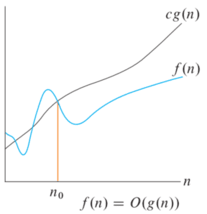
Definition 3.1 (Big-\mathcal O) A function f(n) is said to be \mathcal O(g(n)) if there exist positive constants c and n_0 such that 0\leq f(n) \leq cg(n) \text{ for all }n\geq n_0.

Let us now dissect the definition. In simple terms, Definition 3.1 says that the function f(n) is dominated by g(n), up to a constant multiplier c and after a transient n\geq n_0. See Figure 3.1.

Figure 3.1: Image courtesy Cormen et al. (2009)

Cormen, Thomas H., Charles E. Leiserson, Ronald L. Rivest, and Clifford Stein. 2009. Introduction to Algorithms, Third Edition. 3rd ed. The MIT Press.

Example 3.1 Note that the function 4 + 10n is O(n). To show this, we follow Definition 3.1 assuming that f(n)=4 + 10n and g(n)=n. To fulfil the conditions of the definition, we need to find constants c and n_0.

In our first attempt, we try c=10 to match the multipliers in front of n in the two functions. We immediately realize that f(n)=4 + 10n is still always greater than 10g(n)=10n, which does not look good for the definition.

Our next attempt is to try c=11. So, we compare the functions f(n)=4+10n and 11g(n)=11n. The function cg(n) still does not fully dominate our function f(n) for all n\in\mathbb{N}; see Figure 3.2.

Figure 3.2

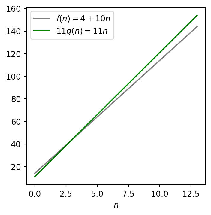
However, this is not a problem for us as long as it dominates after a finite, transient period, i.e., f(n)\leq cg(n) for all n\geq n_0 for some n_0. Existence of such an n_0 is good enough. Well, we can choose n_0=4.

Exercise 3.1 Show that the function 4 + 10n is also O(n^2)! Keep in mind, big-\mathcal O is only an upper bound.

Solution

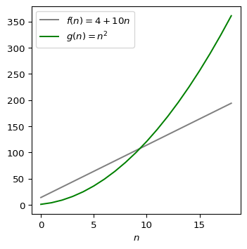
We need to find at least one c and a corresponding n_0 such that 4 + 10n \leq cn^2\text{ for all }n\geq n_0. An obvious choice is c=1 and n_0=10; see Figure 3.3.

Figure 3.3

Exercise 3.2 Show that the function n^2 - 5n + 10 is not O(n).

Solution

Hint: See the plot below.

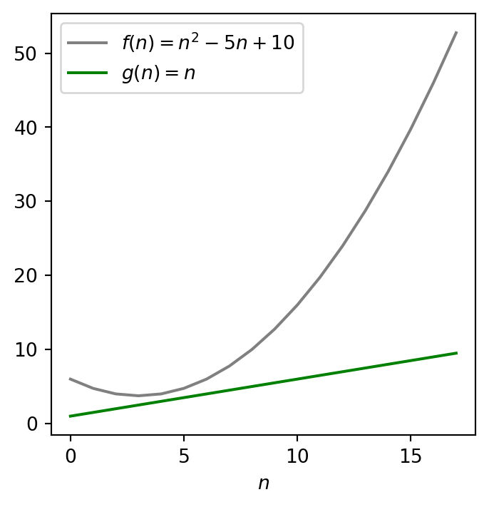
Proving that a function f(n) is not O(g(n)) takes a different a strategy. It amounts to showing that whatever constant c you choose, there is no corresponding transient threshold n_0 such that f(n)\leq cg(n) for all n\geq n_0.

We do this using proof by contradiction. Let us assume the contrary that f(n) is O(g(n)). By Definition 3.1, there must exist positive constants c and n_0 (both independent of n) so that n^2 - 5n + 10 \leq cn\text{ for all }n\geq n_0.

Consequently, n^2 - 5n - cn \leq -10\text{ for all }n\geq n_0.

As a result, n(n - 5 - c) \leq -10\text{ for all }n\geq n_0. Since the right-hand-side is negative (-10), the left-hand-side must also be negative. However, a product can be negative only if exactly one of the terms is negative. We already know that n is positive due to n\geq n_0. Therefore, we must have n - 5 - c < 0\text{ for all }n\geq n_0. Equivalently, n - 5 < c\text{ for all }n\geq n_0. In other words, c is bigger than n-5 for any large n one wishes to choose. This contradicts the fact that c is a constant.

Therefore, we conclude that n^2 - 5n + 10 is not O(n).

Figure 3.4

Exercise 3.3 Check if the functions \sqrt{x} and x^2 are big-\mathcal{O}.

Commonly Used Families

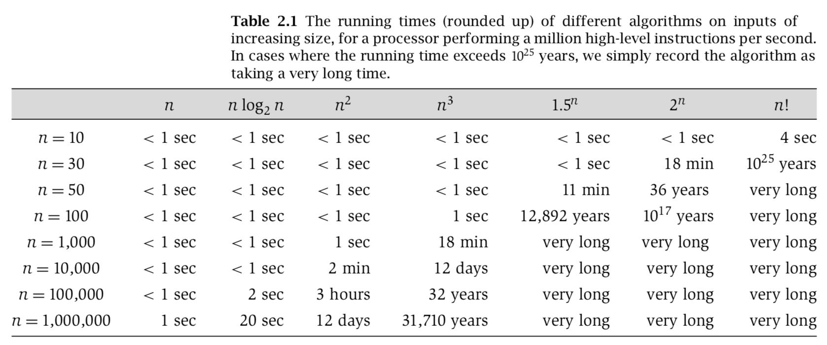
Some of the commonly used families you will come across are:

• O(\lg{n})

• O(n)

• O(n\lg{n})

• O(n^2)

• O(n^3)

• O(2^n)

For a comparison, see Figure 3.5

Figure 3.5: Figure courtesy (Kleinberg and Tardos 2006).

Kleinberg, Jon, and Éva Tardos. 2006. Algorithm Design. Addison Wesley.

Exercise 3.4 Can you think of an algorithm where the running time is in the order of 2^n?

3.2 The Big-\Omega Notation

The big-\Omega notation brings many apparently different looking functions under a common umbrella, by providing an asymptotic lower bound for them. So, big-\Omega notation characterizes an lower bound on the asymptotic behavior. In other words, it says that a function grows no slower than a certain rate, based on the lowest-order term.

The notation is not restricted to only running times T(n) but can be used when considering any general function f(n):\mathbb{N}\to\mathbb{N}. The big-O can also be used, for example, in the context of space-complexity.

Definition 3.2 (Big-\Omega) A function f(n) is said to be \Omega(g(n)) if there exist positive constants c and n_0 such that 0\leq cg(n) \leq f(n) \text{ for all }n\geq n_0.

Exercise 3.5 Show that the function 4 + 10n^2 is \Omega(n). Show that the function is also \Omega(n^2).

Exercise 3.6 Show that the function 4 + 10n^2 is not \Omega(n^3).

A Quick Check using Limit

1. If \lim_{n\to\infty}\frac{f(n)}{g(n)}=0, the the function f(n) is \mathcal O(g(n)).

2. If \lim_{n\to\infty}\frac{f(n)}{g(n)}=\infty, then the function f(n) is \Omega(g(n)).

Exercise 3.7 Can you give an example where a function f(n) is \mathcal O(g(n)), but the limit \lim_{n\to\infty}\frac{f(n)}{g(n)}\neq0.

Exercise 3.8 Can you give an example where a function f(n) is \Omega(g(n)), but the limit \lim_{n\to\infty}\frac{f(n)}{g(n)}\neq\infty.

3.3 Insertion Sort

Now, we will see why big-\mathcal O notation makes sense. Remember big-\mathcal O sets an upper bound on a function. Oftentimes, the best and worst case running times of an algorithm are very different. The notation is used to cover all the different cases. We use the running times of INSERTION-SORT to illustrate the point.

In homework 1, we have already developed and analyzed the selection sort algorithm. An alternative sorting algorithm, known as insertion sort, can outperform SELECTION-SORT on some inputs.

Pseudocode (INSERTION-SORT)

\begin{algorithm} \caption{InsertionSort} \begin{algorithmic} \Procedure{InsertionSort}{$A[0:n-1]$} \For{$i=1$ to $n-1$} \State{$key = A[i]$} \State{▷ Insert $A[i]$ into the sorted sub-array $A[0:i-1]$} \State{$j=i-1$} \While{$j\geq0$ and $A[j]>key$} \State{$A[j+1]=A[j]$} \State{$j=j-1$} \EndWhile \State{$A[j+1]=key$} \EndFor \EndProcedure \end{algorithmic} \end{algorithm}

Exercise 3.9 Demonstrate the correctness of INSERTION-SORT by (dry)-running it on the input A=<5, -2, 0, 1, 6, 3>.

Exercise 3.10 Briefly describe the strategy of INSERT-SORT in plain English.

Solution

Demo

viewof n = Inputs.range([1, 10], {
  value: 5,
  step: 1,
  label: tex`n`
})

{
  move; insert;
  const container = d3
    .create("div")
    .attr("width", width)
    .style("min-height", '100px')
    .style("margin-top", '30px')
    .style("margin-bottom", '30px')
  
  container
    .selectAll(".element")
    .data(A)
    .join("div")
    .attr("class", "element")
    .style("border", (d, id) =>
      id > i ? "3px dashed pink" : "3px solid lightgreen" 
    )
    .style("width", "50px")
    .style("height", "50px")
    .style("padding", "2px")
    .style("text-align", "center")
    .style("display", "inline-block")
    .style("font-size", "20px")
    .style("line-height", "40px")
    .text((d, id ) => !inserted && id == j + 1 ? "↑" : d )
      .append("div")
      .style("position", "absolute")
      .text((d, id) => !inserted && id == j + 1? "🔑=" + key : "");
  return container.node();
}

viewof increment = Inputs.button(i + ' ↦ ' + (i+1), {
  label: tex`\text{Increment } i`,
  value: 0,
  disabled: !sorted || !inserted || i >= n - 1,
  reduce: () => {
    if(sorted && inserted)
      mutable inserted = false;
      mutable i = mutable i + 1;
      mutable key = A[i];
  }
})

viewof move = Inputs.button("j=" + j, {
  value: null,
  label: tex`\text{Move }A[j]`,
  disabled: !(j >= 0 && A[j] > key), 
  reduce: () => {
    if(j >= 0 && A[j] > key) {
        A[j + 1] = A[j];
        mutable j = mutable j - 1;
    }
  }
})

viewof insert = Inputs.button(tex`\text{Insert}`, {
  value: null,
  disabled: !(!inserted && (j < 0 || A[j] <= key)), 
  reduce: () => {
    if(!inserted && (j < 0 || A[j] <= key)) {
        A[j + 1] = key;
        mutable inserted = true;
    }
  }
})

mutable inserted = true;
mutable key = A[i];
mutable i = 0;
mutable j = i - 1;
A = d3.range(n).map((d) => d3.randomInt(-10, 10)());
sorted = {
  move;
  for (let id = 1; id <= i; id++) {
    if (A[id] < A[id - 1]) return false;
  }
  return true;
}

Exercise 3.11 After gaining insights from the above demo, can you guess the best and worst case inputs to INSERTION-SORT?

Solution

The best case input is a sorted array in increasing order. And, the worst case input is a sorted array in decreasing order.

Exercise 3.12 Implement INSERTION-SORT in Python?

Comparison with SELECTION-SORT

In order to compare insertion sort with selection sort, we need to analyze the running time of insertion sort. As we have seen before, we can summarize the computational costs in a table.

We first present the running time for the best input: sorted in increasing order.

Line	Cost	Times
2	c_1	n
3	c_2	n-1
4	c_3	n
5	c_4	n
6	c_5	0
7	c_6	0
9	c_7	n-1

So, T(n)=(c_1 + c_2 + c_3 + c_4 + c_7)n - (c_2 + c_7)=a + bn.

We now present the running time for the worst input: sorted in decreasing order.

Line	Cost	Times
2	c_1	n
3	c_2	n-1
4	c_3	n-1
5	c_4	\sum_{i=1}^{n-1}i
6	c_5	\sum_{i=1}^{n-1}(i - 1)
7	c_6	\sum_{i=1}^{n-1}(i - 1)
9	c_7	n-1

So, \begin{align*} T(n) &=(c_4 + c_5 + c_6)\sum_{i=1}^{n-1} i - (c_5 + c_6) \sum_{i=1}^{n-1}1 \\ & \quad+ (c_1 + c_2 + c_3 + c_7)n - (c_2 + c_7) \\ &=(c_4 + c_5 + c_6)\frac{(n-1)n}{2} - (c_5 + c_6)(n-1) \\ & \quad+ (c_1 + c_2 + c_3 + c_7)n - (c_2 + c_7) \\ &=a + bn + cn^2. \end{align*}

In order to cover both cases, we can say that the running time of INSERTION-SORT is \mathcal O(n^2).

3.4 Merging Sorted Subarrays

Merging two sorted arrays is a crucial step used in MERGE-SORT, a recursive way to sort an array. For this exercise, we take a thorough look at this subroutine.

Given an array A[0:n-1] and three indices p,q,r from it such that p\leq q<r. The procedure assumes that the two adjacent subarrays A[p:q] and A[q+1:r] are already sorted. It merges them to form a single sorted subarray that replaces the current subarray A[p:q]. Here is the pseudocode.

\begin{algorithm} \caption{Merge} \begin{algorithmic} \Procedure{Merge}{$A[0:n-1], p, q, r$} \State{$n_L=q-p+1$}\Comment{length of $A[p:q]$} \State{$n_R=r-q$}\Comment{length of $A[q+1:r]$} \State{$L[0:n_L-1]$ and $R[0:n_R-1]$ be two new arrays} \For{$i=0$ to $n_L-1$}\Comment{Copy $A[p:q]$ into $L[0:n_L]$} \State{$L[i]=A[p+i]$} \EndFor \For{$j=0$ to $n_R-1$}\Comment{Copy $A[q:r]$ into $R[0:n_R]$} \State{$R[j]=A[q+j+1]$} \EndFor \State{$i=0$}\Comment{$i$ indexes the smallest remaining element in $L$} \State{$j=0$}\Comment{$j$ indexes the smallest remaining element in $R$} \State{$k=p$}\Comment{$k$ indexes the location in $A$ to fill} \While{$i<n_L$ and $j<n_R$} \If{$L[i]\leq R[j]$} \State{$A[k]=L[i]$} \State{$i=i+1$} \Else \State{$A[k]=R[j]$} \State{$j=j+1$} \EndIf \State{$k=k+1$} \EndWhile \State{▷ Having gone through one of $L$ and $R$ entirely, copy the remainder of the other to the end of $A[p:r]$.} \While{$i<n_L$} \State{$A[k]=L[i]$} \State{$i=i+1$} \State{$k=k+1$} \EndWhile \While{$j<n_R$} \State{$A[k]=R[j]$} \State{$j=j+1$} \State{$k=k+1$} \EndWhile \EndProcedure \end{algorithmic} \end{algorithm}

Demo

viewof n1 = Inputs.range([5, 15], {
  value: 10,
  step: 1,
  label: tex`n`
})
viewof p = Inputs.range([0, n1 - 1], {
  value: 0,
  step: 1,
  label: tex`p`
})
viewof q = Inputs.range([p, n1 - 1], {
  value: p+1,
  step: 1,
  label: tex`q`
})
viewof r = Inputs.range([q+1, n1 - 1], {
  value: n1 - 1,
  step: 1,
  label: tex`r`
})

B = d3.range(n1).map((d) => d3.randomInt(-10, 10)());
L = d3.range(q - p + 1).map(d => "▢");
R = d3.range(r - q).map(d => "▢");
mutable i1 = 0;
mutable j1 = 0;
mutable k1 = p;
mutable sorted1 = false;

viewof sort = Inputs.button('sort subarrays', {
  value: null,
  disabled: sorted1,
  reduce: () => {
    if(!sorted1) {
      B.splice(p, q - p + 1, ...B.slice(p, q + 1).sort(function(a, b) {
        return a - b;
      }));
      B.splice(q + 1, r - q, ...B.slice(q + 1, r + 1).sort(function(a, b) {
        return a - b;
      }));
      L.splice(0, L.length, ...B.slice(p, q + 1));
      R.splice(0, R.length, ...B.slice(q + 1, r + 1));
      mutable sorted1 = true;
    }
  }
})

{
  sort; increment1;
  const container = d3
    .create("div")
    .attr("width", width)
    .style("min-height", '100px')
    .style("margin-top", '30px')
    .style("margin-bottom", '30px')
  
  container
    .selectAll(".element")
    .data(B)
    .join("div")
    .attr("class", "element")
    .style("border", "3px solid lightgray")
    .style("border-style", (d, id) =>
      id >= p && id <= r ? "solid" : "dashed" 
    )
    .style("border-color", (d, id) =>
      sorted1 ? "lightgray" : id >= p && id <= r ? id <= q ? "pink" : "lightgreen" : "lightgray" 
    )
    .style("width", "50px")
    .style("height", "50px")
    .style("padding", "2px")
    .style("text-align", "center")
    .style("display", "inline-block")
    .style("font-size", "20px")
    .style("line-height", "40px")
    .text((d, id ) => d )
      .append("div")
      .style("position", "absolute")
      .text((d, id) => id == p ? "p=" + p : id == q ? "q=" + q : id == r ? "r=" + r : "" )
      .append("div")
      .style("position", "absolute")
      .style("transform", "translateY(-300%)")
      .text((d, id) => sorted1 ? id == k1 ? "k=" + k1 : "" : "");
  return container.node();
}

{
  sort; increment1;
  const container = d3
    .create("div")
    .attr("width", width)
    .style("min-height", '100px')
    .style("margin-top", '20px')
    .style("margin-bottom", '30px')
  
  container
    .selectAll(".left")
    .data(L)
    .join("div")
    .attr("class", "left")
    .style("border", "3px solid pink")
    .style("width", "50px")
    .style("height", "50px")
    .style("padding", "2px")
    .style("text-align", "center")
    .style("display", "inline-block")
    .style("font-size", "20px")
    .style("line-height", "40px")
    .style("margin-right", (d, id) => id == L.length - 1 ? "20px" : "0px")
    .text((d, id ) => d )
      .append("div")
      .style("position", "absolute")
      .text((d, id) => id == i1 ? "i=" + i1 : "" );

  container
    .selectAll(".right")
    .data(R)
    .join("div")
    .attr("class", "right")
    .style("border", "3px solid lightgreen")
    .style("width", "50px")
    .style("height", "50px")
    .style("padding", "2px")
    .style("text-align", "center")
    .style("display", "inline-block")
    .style("font-size", "20px")
    .style("line-height", "40px")
    .text((d, id ) => d )
      .append("div")
      .style("position", "absolute")
      .text((d, id) => id == j1 ? "j=" + j1 : "" );
  return container.node();
}

viewof increment1 = Inputs.button('increment k', {
  value: null,
  disabled: !(sorted1 && k1 <= r),
  reduce: () => {
    if(sorted1 && k1 <= r) {
      if(i1 < L.length && j1 < R.length) {
        if(L[i1] <= R[j1]) {
          B[k1] = L[i1];
          mutable i1 = mutable i1 + 1;
        }
        else {
          B[k1] = R[j1];
          mutable j1 = mutable j1 + 1;
        }
      }
      else if(i1 < L.length) {
        B[k1] = L[i1];
        mutable i1 = mutable i1 + 1;
      }
      else if(j1 < R.length) {
        B[k1] = R[j1];
        mutable j1 = mutable j1 + 1;
      }
      mutable k1 = mutable k1 + 1;
    }
  }
})

Exercise 3.13 Implement MERGE (Algorithm 2) in Python.

Exercise 3.14 Describe the running time of MERGE (Algorithm 2) in terms of n, the total number of elements in the subarray A[p:r].

Solution

The running time is T(n)=O(n), where n = r - p + 1.

Computer virus. Image courtesy Timothy Young